

Biomolecular Hydration Analysis Package
|
IntroductionBenchmarkBuried watersProtocolPreprocessingAtom centric approachSolvent densityResidence timeDistance of closest waterAnalysisDownload and InstallHow to run the programsScripts to compute hydration propertiesScripts to process the outputGeneral pointsReferencesContactIntroduction‘JAL’ is a collection of python programs for fast and accurate computation of hydration properties in MD trajectories. Programs calculate solvent density, residence time, buried waters and closest water distance. Additionally, included is a novel algorithm for computing buried water in an MD trajectory.Kinds of output are available- graphic and textual. Textual output involves a summary file containing the quantification of hydration properties. Some textual files, for instance .pdb file, can be readily loaded in pymol or can be plotted using xmgrace. These post processing scripts are provided in the Scripts section which allows an insightful visualization of the hydration property. Novelty of the approach lies in the way the calculations are performed. Instead of a traditional grid based approach, we track solvent molecules based on their proximity to the solute to compute solvation properties (More details in the Reference). Though originally designed for hydration analysis of protein, the scripts can also be used for hydration analysis of small molecules, nucleic acids or any other macromolecules. BenchmarkBuried watersComputation of buried waters were benchmarked against bovine trypsin inhibitor (PDB id- 4PTI (1.5Å, REF)). There are 4 buried waters in the protein and our program correctly identified these buried waters (Figure 1) in crystal structure as well as in MD trajectory.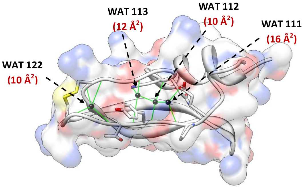
Figure 1: Buried water in the crystal structure of bovine trypsin inhibitor. [back to top] ProtocolThis section provides a general overview of the approaches used to compute hydration properties in structural ensemble of biomolecules. More detailed explanation can be found in the reference paper.PreprocessingThe 1st step in using the ‘JAL’ programs to compute hydration properties is to preprocess the trajectory using the preprocessing script (preprocess.py). This program reads a single MD trajectory in PDB format (multiple frames appended in one file). The aim of preprocessing the trajectory is to reduce the size of system in order to reduce the number of computations. Preprocessing involves the following two steps- (1) stripping all the hydrogen atoms in the system, and (2) stripping all the solvent atom beyond user defined cut off (default = 3.5 Å which marks the 1st solvation shell). Additionally, the user might be interested in computing hydration properties only for a subset of solute atoms/residues. These can be specified too so that other solute atoms and their vicinal water molecules can be stripped.The output of preprocessing (a trimmed MD trajectory files) is the input for the subsequent programs that compute hydration metric. The reduced size of the system (solute + solvent) enables to rapidly compute hydration metrics. [back to top] Atom centric approachSolvent properties (solvent density, residence time, closest water distance) are computed by tracking water molecules within a sphere of 3.5 Å from the reference (non-hydrogen protein) atoms in each snapshot of the input structural ensemble. The 3.5 Å cut off is optimal because it is the maximum hydrogen bond donor to hydrogen bond acceptor distance for a hydrogen bond and there are rarely more than one water molecule within this sphere.This approach of computing the solvent properties is different from a grid based approach. A grid based approach requires creating a grid over the water box and then counting the number of the solvent molecules within each grid box (usually of 0.5 Å dimension); we use a protein centric approach where we monitor the protein (non-hydrogen) atoms that interact with the solvent (water oxygen). Although, this approach is computationally more expensive than the grid based approach, our method provides insightful representations of the data as discussed in the results section. This also makes sense, in that the solvation around a protein is a function of the chemistry and topology of the protein surface. Representing solvent density as grid boxes in 3D (as represented by the ‘grid’ function in Amber’s ptraj module for instance) obscures the identity of the solute atoms that are critical for the respective solvent densities around the solute. Additionally, the grid based approach is extremely sensitive to solute dynamics and therefore affects the accuracies of the solvent properties computed in the 3D grids in cases where the solute is very flexible and/or undergoes major conformational changes; our atom centric approach does not suffer from these limitations. Furthermore, just like the grid based method provides a hydration measure (e.g. solvent density) that is properly normalized by voxel volume, has clear interpretation, and as such is transferable between different locations and different systems; the hydration measure computed using atom centric approach, too, is transferrable if the same color spectrum scale is used (as shown in the figure in Section V ‘How to run the programs’ of the manual). [back to top] Solvent densityIt measures the extent of hydration of an atom or group of atoms on solute. The program computes the number of times a site on solute is hydration (water molecule < 3.5 Å of the reference solute atom). Computations can be done for a subset of solute atoms of all the solute atoms. This metric is measured as percent solvation (percent of the simulation time a site on solute is hydrated) using the following formulation-
W is the any water oxygen (irrespective of the ID) at a given instance of time and Δt is the time interval between two successive snapshots of the MD trajectory. Here, Δt is 100 ps. Value of γ is 1 if W(t) = W(t + Δt) and 0 otherwise. [back to top] Residence timeThe residence time is defined as the length of time a distinct water molecule stays continuously within 3.5 Å of the solute site. This produces a list of residence time values for that water at that site across the MD trajectory. The summation of all such values at a site gives the total residence time, the average of this gives the average residence time and the maximum value from this list is reported as the maximum residence time (the total residence time will depend on the length of the trajectory). Effectively, the program computes the residence time autocorrelation function P(t) (as also done previously (De Simone et al., 2005) but does not fit an exponential or multi exponential model. It is an estimate of how stable/buried/trapped a water molecule is at a particular site.
[back to top] Buried watersOne of the utilities of the package is to compute water molecules that are buried in the protein core. These (buried) waters have little solvent accessibility and are referred to as buried waters. Buried waters are computed using a novel methodology based on iterative calculations of Solvent Accessible Surface Area (SASA) of water molecules and deleting those waters which have SASA more than zero after every iteration (analogous to ‘evaporating’ waters on the protein surface) (shown in the figure below). Ultimately waters left with SASA value of zero are the ones which are present in the protein interior, and are thus deemed to be buried. SASA is computed using the rolling ball algorithm.
Figure 2: Schematic diagram to demonstrate the computation of buried waters in an MD trajectory. The program to compute buried waters takes as input an MD trajectory of the solute (protein) with the water box. For every frame, the program computes the SASA of all the heavy atoms in the system using the rolling ball algorithm 45. This entails rolling a probe of the size of a water molecule (radius of 1.4 Å) on the system (protein + water box). In the next step, all the waters with a non-zero SASA value are deleted. Computation of SASA of all heavy atoms followed by deletion of the waters with a non-zero SASA value is iterated till only waters with a SASA value of zero (buried waters) are left; this value can be changed to non-zero values to reflect almost completely buried waters, etc. 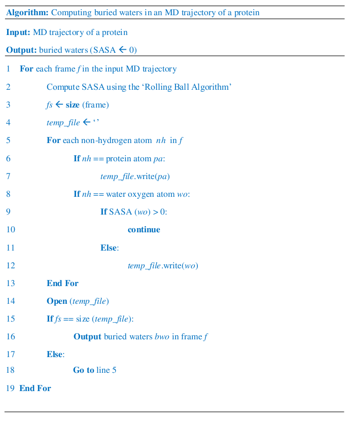
[back to top] Distance of closest waterIt computes the distance between a solute atom and the closest solvent molecule. The metric estimates the accessibility of a site on the solute to the water and hence provides a likely estimate of the strength of the interaction.[back to top] AnalysisOutput is provided as summary in text format and also as files that can be readily visualized in an easy, interactive and intuitive manner. We try to describe the output for some of the programs here-Summary outputThe solvent density and residence time values computed by the wat_resi_exchange.py are summarized in a file in the format shown below-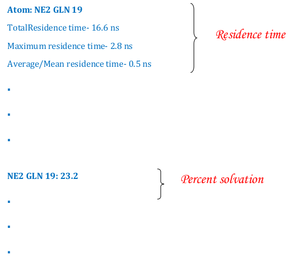
[back to top] Mapping the hydration property on a structure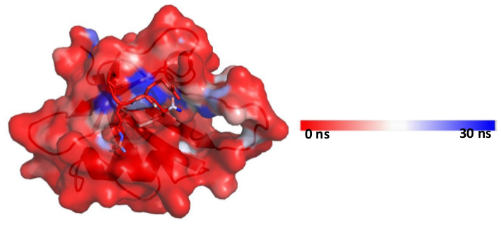
[back to top] Buried waters output1)Buried water vs frame no.Output in text format that can be plotted >> xmgrace buried-wat_Vs_frame-no 2)Buried water IDs in each frame 1 : [242, 244, 245, 8172] 2 : [244, 245, 8172] 3 : [242, 244, 245, 249, 250, 511, 8172, 242, 244] 4 : [242, 244, 245, 249, 250, 8172] 5 : [241, 245, 246, 249, 252, 253, 266, 284, 8172] 6 : [242, 244, 245, 249, 250, 8172] 7 : [242, 244, 245, 247] 8 : [242, 244, 245, 247, 249, 8172] 9 : [242, 245, 247, 249] 10 : [242, 244, 245, 247, 249, 228] [back to top] A trajectory with only buried watersThe program also produces a trajectory, in pdb format, of the solute and only the buried waters. This trajectory can be visualized in PyMOL.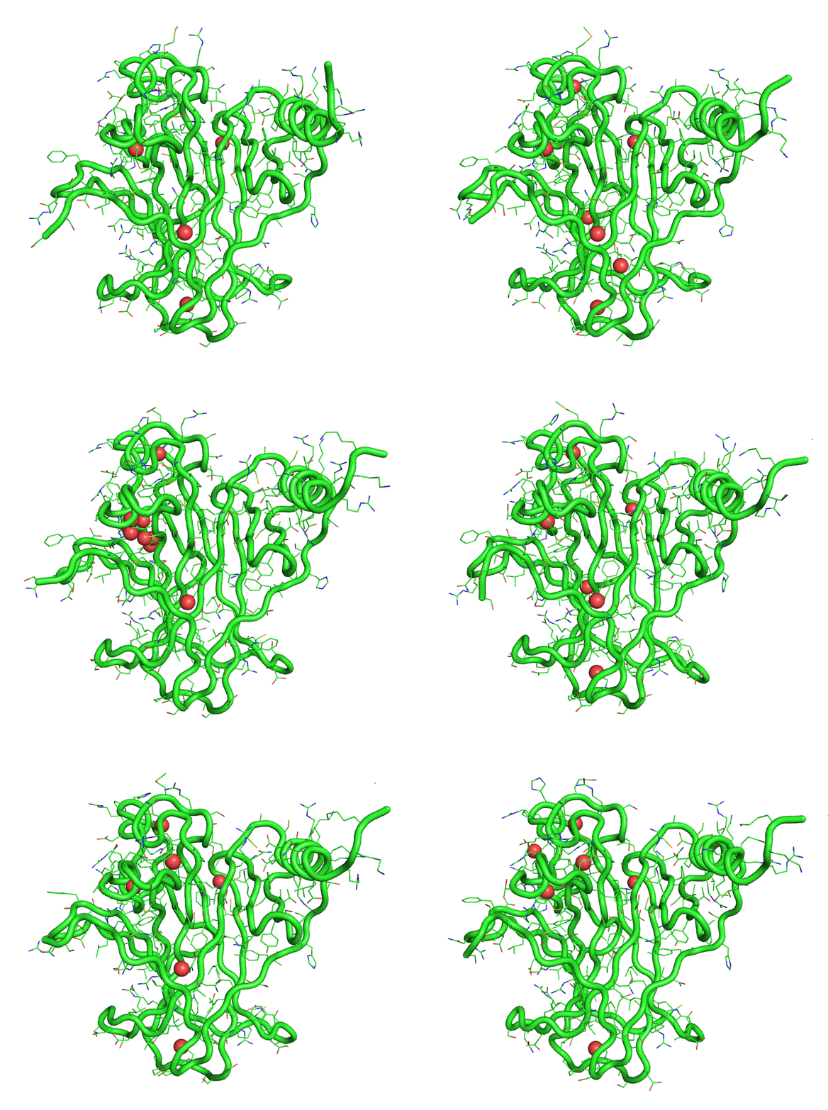
[back to top] Time series of solvent exchanges at a solute site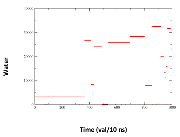
[back to top] Download and InstallThe ‘JAL’ package is available for free download. Please click here to download the standalone version of the software package – Jal.tar.gzRefer the 'jal_readme' for instructions to download JAL and install required dependencies on your machine [back to top] How to run the programsScripts to compute hydration propertiesInput files are highlighted and the running times of scripts are shown in the images.1. preprocess1.py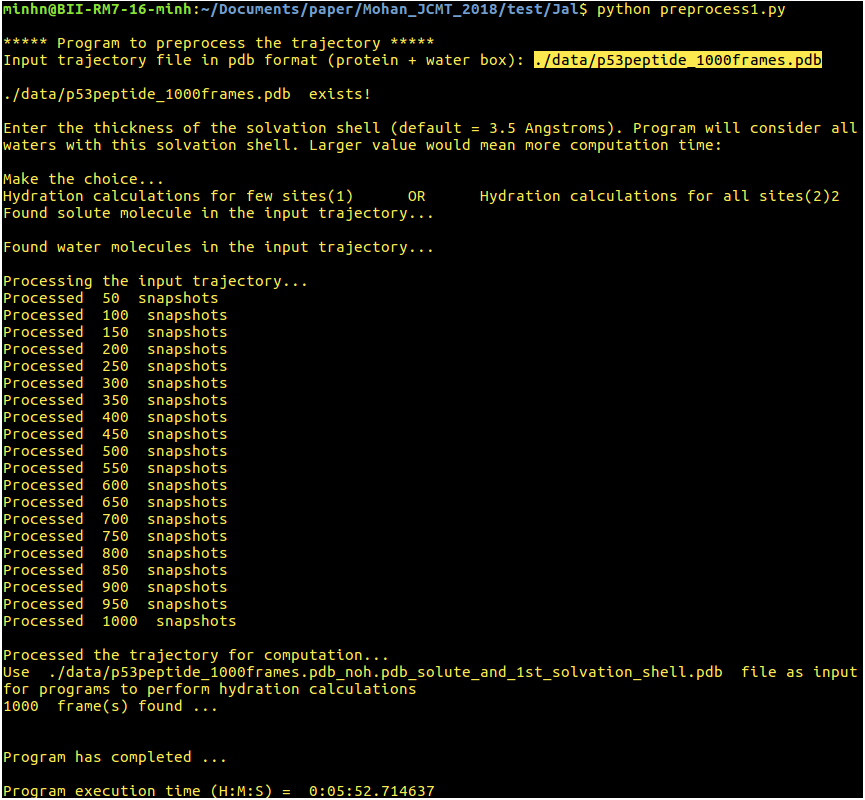
[back to top] 2. wat_resi_n_exchange_all_pdb_sites.py
[back to top] 3. wat_resi_n_exchange.py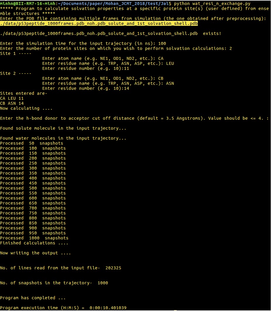
[back to top] 4. buried_wat_using_sasa5.py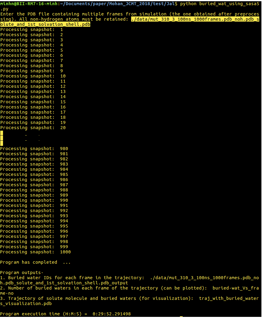
[back to top] 5. closest_wat_distance.py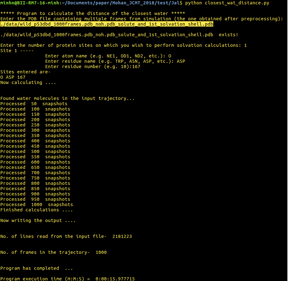
[back to top] Scripts to process the output1. Color protein according to solvation/residence time of waters in an MD trajectory in PyMOL- Load ‘’ or ‘’ in pymol- Type the following command in pymol spectrum b, red_white_blue, minimum=0, maximum=100 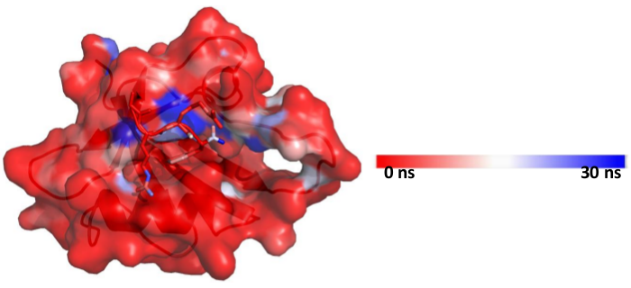
The user can change the minimum and maximum values as per required [back to top] 2. Visualize the rate of exchange of water at a particular site on protein in xmgrace- Load the file in xmgrace> xmgrace p53dbd_1000frames.pdb_noh.pdb_solute_and_1st_solvation_shell.pdb_N-CYS-90_water_id 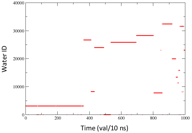
- Customize the visualization in xmgrace [back to top] General points[back to top] References[back to top] ContactEmail: chandra@bii.a-star.edu.sgTechnical details: Minh N. Nguyen Email: minhn@bii.a-star.edu.sg Group: Atomistic Simulations and Design in Biology Institute: Bioinformatics Institute A*STAR [back to top] |